From ζ(2) to Π. The Proof.

30 Mar 2017

Introduction

For some reason, the sum of the inverse of the square of all natural positive numbers is $\pi^2/6$. This sum is also called the function ζ(2) of Riemann and the search of its value the Basel problem.

$$\zeta(2) \quad = \quad \sum_{n\geq1} \frac{1}{n^2} \quad = \quad \frac{\pi^2}{6}$$

In this article, I cover the proof of this equality step by step. For understanding this proof, no advanced mathematical knowledge is required, the advanced topics required for the proof will be explained further ahead.

Good luck.

Double Integral

For this proof we are going to start from this double integral of a function of two variables.

$$\int_{0}^{1} \int_{0}^{1} x^{n-1} y^{n-1} \,dx \,dy$$

Our first task is to solve this double integral. How? It’s easier than it looks. Basically, we are going to integrate first with respect to x and then with respect to y. So we could write the expression this way:

$$\int_{0}^{1} \left( y^{n-1} \int_{0}^{1}x^{n-1} \,dx \,dy \right)$$

I assume that you can solve these integrals. Surprisingly, we obtain:

$$\frac{1}{n} \cdot \frac{1}{n} = \frac{1}{n^2}$$

I hope that now that weird double integral of the beginning looks more related with our proof. So let’s try to simplify the expression when we have our series.

$$\frac{1}{n^2} = \int_{0}^{1} \int_{0}^{1} (xy)^{n-1} \,dx \,dy \Rightarrow \sum_{n\geq1} \frac{1}{n^2} = \sum_{n\geq1} \int_{0}^{1} \int_{0}^{1} (xy)^{n-1} \,dx \,dy$$

Because of integrals properties the sum of integrals is equal to the integral of the sum:

$$\sum_{n\geq1} \int_{0}^{1} \int_{0}^{1} (xy)^{n-1} \,dx \,dy = \int_{0}^{1} \int_{0}^{1} \sum_{n\geq1} (xy)^{n-1} \,dx \,dy$$

Now, our function is a geometric series, but we need to transform the power n-1 to n, and start from 0 instead of 1.

$$\sum_{n\geq1} (xy)^{n-1} = \sum_{n\geq0} (xy)^{n}$$

Ok, now we have a geometric series than can be easily simplified. Moreover, we know that the term xy it’s going to be less than 1, because the limits of integration go from 0 to 1. Therefore x and y will take values from 0 to 1.

Fortunately, a geometric series whose term’s absolute value is lower than 1 can be simplified this way:

$$\sum_{n\geq0} (xy)^{n} = \frac{1}{1-xy}$$

Hence we have the following equality:

$$\sum_{n\geq1} \frac{1}{n^2} = \int_{0}^{1} \int_{0}^{1} \frac{1}{1-xy} \,dx \,dy$$

Overview of functions of two variables

I told you that advanced mathematical knowledge wasn’t required. However, we’ve been working with double integrals and functions of two variables. So, what’s going on? Well, unfortunately, there is no way to understand this proof without certain concepts, so we’ll take a look at these concepts.

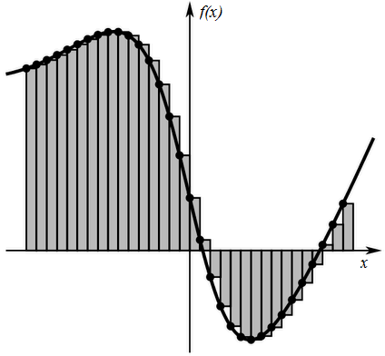
Let’s start with the original concept of integral. An integral can be imagined as a sum of a lot of rectangles with base dx, and height f(x):

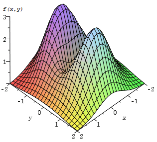
But if we have a function of two variables the idea changes.

First of all, unlike a function of one variable, we can’t represent it like a 2D curve. Now, for the function f(x,y) we can obtain infinite values of the function with the same x changing the y and vice versa. So if we represent it, we’ll see something like a mesh or a surface. Something like this example (not our function).

And now, instead of calculating areas we will calculate the volume under the surface defined by the function. Because the integral is definite, we will calculate the volume of the function in a certain area. In our integral both variables are delimited between 0 and 1, so we are calculating the volume of the function under a square of vertices (0,0) (0,1) (1,0) (1,1).

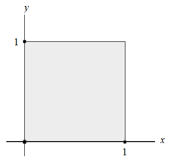
To imagine geometrically how it works, now instead of rectangles with base dx and height f(x), we calculate a sum of prisms with base dxdy and height f(x,y).

Change of variables

In order to obtain our appreciated proof we will integrate by substitution. In this case, we are doing a a linear change of coordinates. Instead of x and y we will work with u and v. And these new variables have the following values:

$$u(x,y) = \frac{x+y}{2} \quad v(x,y) = \frac{-x+y}{2}$$

We can also express x and y in terms of u and v:

$$x(u,v) = u-v \quad y(u,v) = u+v$$

Ok, so what’s next? Well, actually we have to complete three main tasks. All these things are also necessary when working with one variable functions but in that case many things are simplified and look trivial.

The 3 things that we have to change are:

• Function $\frac{1}{1-xy}$
• Differential $\,dx\,dy$
• Limits of Integration $\int_{0}^{1} \int_{0}^{1}$

All the steps can be explained with the following intimidating expression:

$$\int \int_{S} f(x(u,v),y(u,v)) \left|\frac{d(x,y)}{d(u,v)}\right|\,du\,dv$$

Function

This is the easiest and best known step. All we have to do is to replace x and y with their values expressed with respect to u and v.

$$f(x,y) = \frac{1}{1-xy} = \frac{1}{1-(u-v) \cdot (u+v)}$$

It can be simplified to:

$$f(x,y) = \frac{1}{1-u^2+v^2}$$

Differential

Because we have changed the variables of the function, we can’t keep our old differentials. Therefore we need to find a way to express du dv with respect to dx dy. Something like this.

$$\,du\,dv = |J|\,dx\,dy$$

Fortunately or unfortunately, someone already thought about it and developed the Jacobian Determinant (J). We must notice that du and dv depend on how x and y derive, this is because both are expressed with respect to x and y, and vice versa.

$$x(u,v) = u-v \quad y(u,v) = u+v$$

That’s the reason why we are going to work with partial derivatives. Don’t worry, is just to derive with respect to a certain variable. For example, the partial derivative of x with respect to u can be written this way:

$$\frac{ \partial x}{ \partial u}$$

And its result is the derivative of the function that express x with respect to u and v but considering v as a constant.

$$\frac{ \partial (u-v)}{ \partial u} = 1-0 = 1$$

So finally, the J that we are looking for is the following determinant:

$$J = \begin{vmatrix} \frac{ \partial x}{ \partial u} & \frac{ \partial x}{ \partial v}\\ \frac{ \partial y}{ \partial u} & \frac{ \partial y}{ \partial v}\\ \end{vmatrix} = \begin{vmatrix} 1 & -1\\ 1 & 1\\ \end{vmatrix} =2$$

Hence we can substitute the differentials:

$$\,dx\,dy = 2\,dv\,du \Rightarrow \frac{2\,dv\,du}{1-u^2+v^2}$$

Limits of Integration

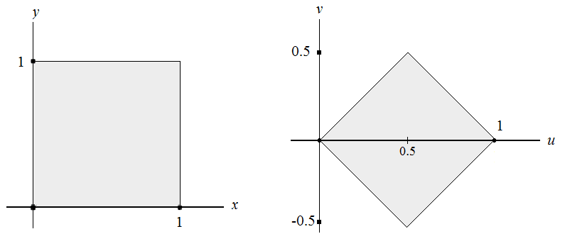
Finally, because we have changed the variables we must change the limits of integration according to the new variables. You may remember that our limits of integration represent a square with vertices (0,0) (0,1) (1,0) (1,1). Ok, if we change the value of these vertices using the variables equivalence we obtain:

$$(x,y) \Rightarrow (u,v) \\ (0,0) \Rightarrow (0,0) \quad (1,1) \Rightarrow (1,0) \\ (0,1) \Rightarrow \left(\frac{1}{2},\frac{1}{2}\right) \quad (1,0) \Rightarrow \left(\frac{1}{2},-\frac{1}{2}\right)$$

So now, we have a rotated and scaled square:

But we have to figure out how to express these new limits. First of all we can notice that if we split the new square in two parts, above and below edge u, the function values are equal in both parts. Why?

Basically, because u and v are squared in the function, so the function will produce the same values no matter if the variables are positive or negative. So we will calculate only the upper part and multiply by 2. And to make it easier, we will split the upper part in two parts.

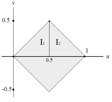
The limits of I₁ and I₂ in the u edge are [0,1/2] and [1/2,1] respectively. The tricky part is finding the limits of v. Well, fortunately we can represent the value of v as a function of u, actually, the limits of v is the function u in I₁, and 1-u in I₂. So our new limits of integration are:

$$2\int_{0}^{1/2} \int_{0}^{u} + 2\int_{1/2}^{1} \int_{0}^{1-u}$$

New Expression

After all this long reasoning we have the following identity:

$$\int_{0}^{1} \int_{0}^{1} \frac{1}{1-xy} \,dx \,dy = \\ 2 \cdot 2\int_{0}^{1/2} \int_{0}^{u} \frac{dv\,du}{1-u^2+v^2} + 2 \cdot 2\int_{1/2}^{1} \int_{0}^{1-u} \frac{dv\,du}{1-u^2+v^2}$$

Arctangent is the key

We will solve our integrals using the integral of arctangent:

$$\int \frac{dx}{a^2+x^2} = \frac{1}{a} arctan \left( \frac{x}{a} \right) + C$$

Therefore, if we solve the first integral and apply the fundamental theorem of calculus we obtain:

$$4\int_{0}^{1/2} \frac{1}{\sqrt{1-u^2}} \cdot arctan \left( \frac{u}{\sqrt{1-u^2}} \right) du + \\ 4\int_{1/2}^{1} \frac{1}{\sqrt{1-u^2}} \cdot arctan \left( \frac{1-u}{\sqrt{1-u^2}} \right) du$$

This is great. You don’t know yet but we have the integral of a function multiplied by its derivative. We will define new variables to simplify it:

$$a(u) = arctan \left( \frac{u}{\sqrt{1-u^2}} \right) \quad a'(u) = \frac{u}{\sqrt{1-u^2}}$$

And for the second part we have:

$$b(u) = arctan \left( \frac{1-u}{\sqrt{1-u^2}} \right) = arctan \left(\sqrt{\frac{1-u}{1+u}} \right) \\ b'(u) = -\frac{1}{2}\frac{1}{\sqrt{1-u^2}}$$

If we replace in the expression we get:

$$4\int_{0}^{1/2} a'(u)a(u)\,du + 4\int_{1/2}^{1} -2 \cdot b'(u)b(u)\,du$$

But if we use the following property of integrals everything can be easily simplified:

$$\int_{a}^{b} f'(x)f(x) \,dx = \left[ \frac{1}{2}f(x)^2 \right]_{a}^{b} = \frac{1}{2}f(b)^2- \frac{1}{2}f(a)^2$$

Therefore we obtain:

$$2\left[a(u)^2 \right]_{0}^{1/2} - 4\left[b(u)^2 \right]_{1/2}^{1} = \\ 2 \cdot a(1/2)^2-2 \cdot a(0)^2-4 \cdot b(1)^2+4 \cdot b(1/2)^2$$

Finally, if we use some trigonometric properties to simplify the result of the functions we get:

$$2\left(\frac{\pi}{6}\right)^2 - 0 - 0 + 4\left(\frac{\pi}{6}\right)^2 = \frac{\pi^2}{6}$$

Hallelujah! $$\zeta(2) \quad = \quad \sum_{n\ge1} \frac{1}{n^2} \quad = \quad \frac{\pi^2}{6} \quad \#$$

Acknowledgement

I want to thank Dr. F. Guil Asensio and Dr. G.M. Diaz-Toca their help for understanding the concepts covered in this article, a computer scientist like me couldn’t have ever understand it without their help.

References

• Apostol, Tom M. A (1983) Proof that Euler missed: evaluating Zeta(2) the easy way. Math. Intelligencer 5, no. 3, 59–60.
• Aigner, M. and Ziegler, G.M. (2014), Proofs from The Book, Springer. Pages 53-60.
• Chapman, R. (2003) Evaluating Zeta(2)
• Alvárez, L. and Martínez A. Cálculo integral de funciones de varias variables.